卡内基梅隆的数据库课程-2
课程地址
https://15445.courses.cs.cmu.edu/fall2021/schedule.html
Query Execution
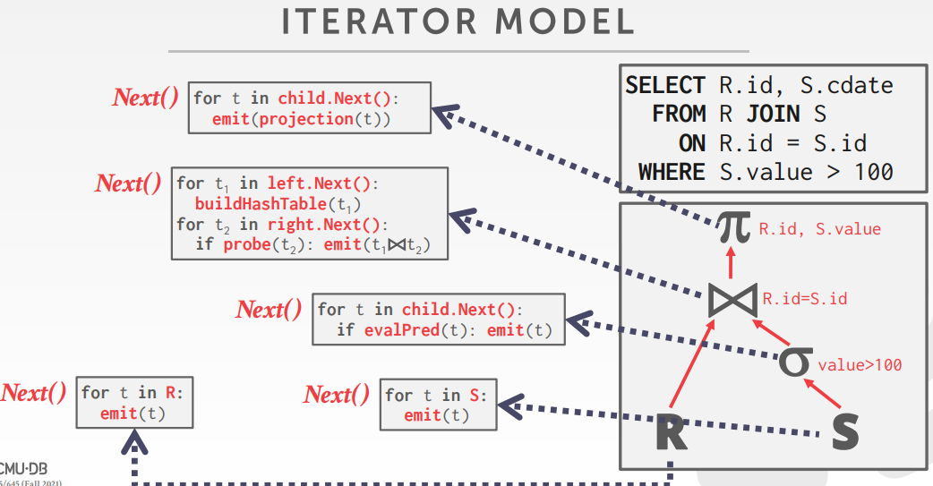
A DBMS’s processing model defines how the system executes a query plan.
- Different trade-offs for different workloads
- Iterator Model,查询计划算子要实现 next()函数
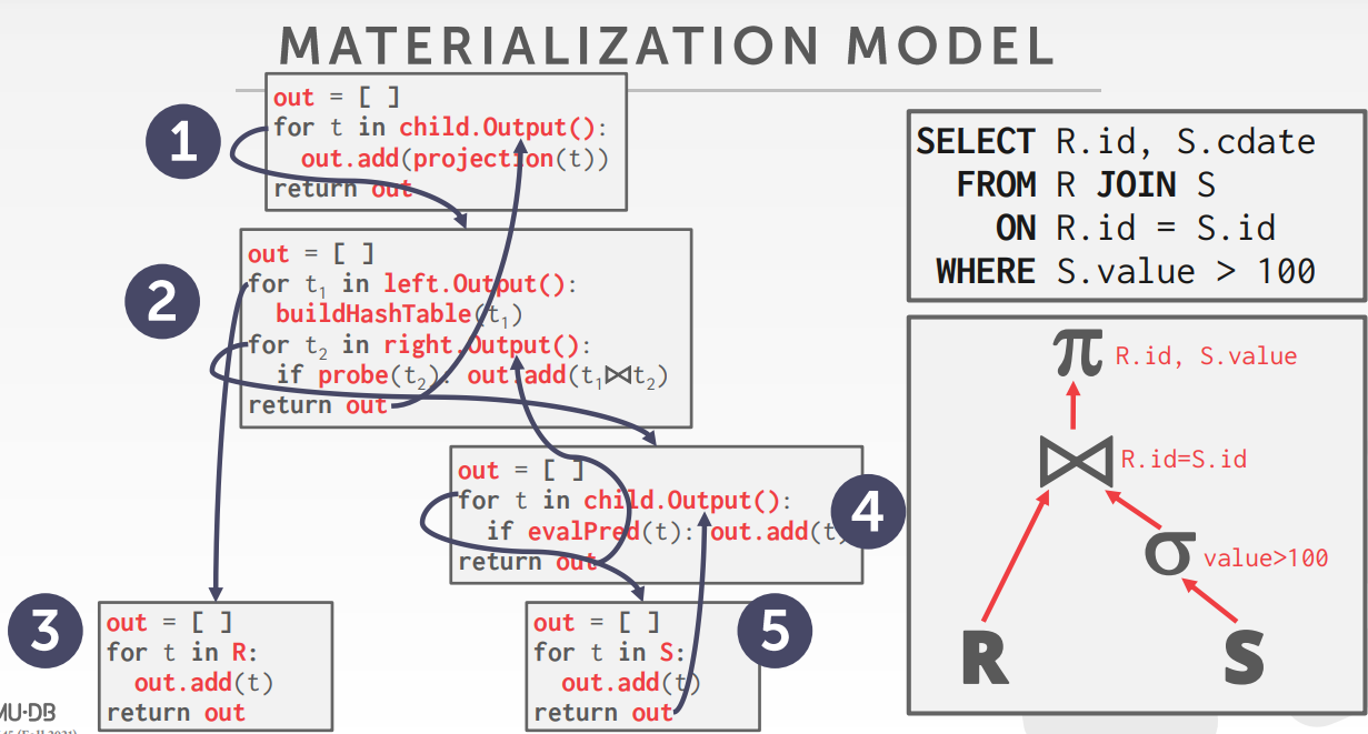
- Materialization Model,
- 物化模式,处理所有输入一次,发射输出一次,物化输出为单个结果,可以返回物化行或者单个列
- 物化模式对 OLTP比较友好,因为只需要访问小数量tuple一次
- 物化模式对OLAP不友好,因为有大数量的中间结果
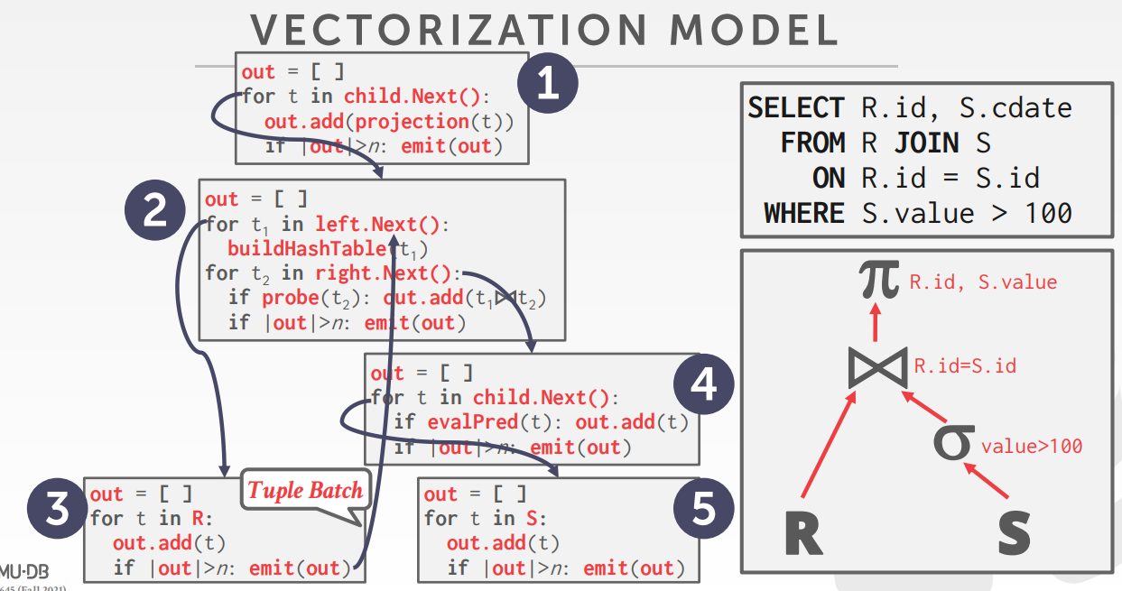
- Vectorized / Batch Model,类似火山模型,一次返回多个值,返回size依赖硬件或查询属性
- 对OLAP友好,因为每个操作减少了很多函数调用,可以支持向量化SIMD指令,处理一批tuple
查询计划处理方向
- top-to-buttom
- Start with the root and “pull” data up from its children.
- Tuples are always passed with function calls.
- Bottom-to-Top
- Start with leaf nodes and push data to their parents.
- Allows for tighter control of caches/registers in pipelines.
access methods
- sequential scan
- index scan
- multi-index、 bitmap scan
sequential scan
|
|
Sequential Scan Optimizations,基本上是最差的方式
- Prefetching
- Buffer Pool Bypass
- Parallelization
- Heap Clustering
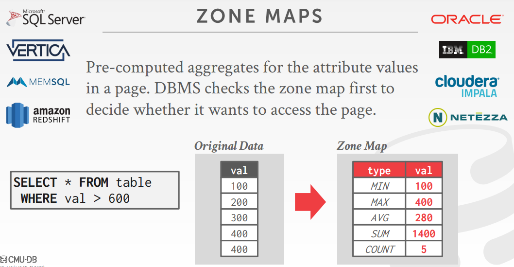
- Zone Maps
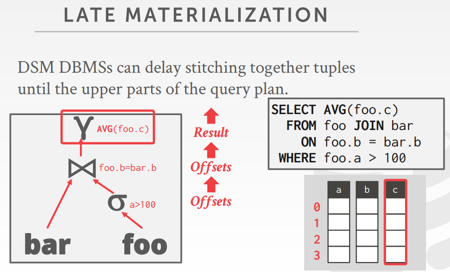
- Late Materialization
zone map,提前预聚合
延迟物化,在查询计划的上面才将元组做拼接
index scan
Which index to use depends on:
- What attributes the index contains
- What attributes the query references
- The attribute’s value domains
- Predicate composition
- Whether the index has unique or non-unique keys
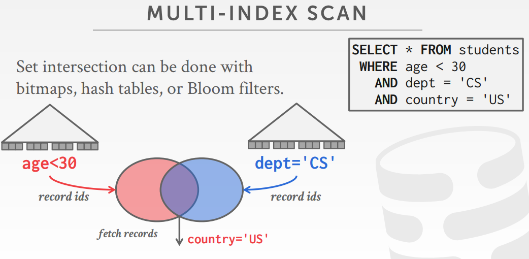
multi-index scan
If there are multiple indexes that the DBMS can use for a query:
- Compute sets of Record IDs using each matching index.
- Combine these sets based on the query’s predicates(union vs. intersect).
- Retrieve the records and apply any remaining predicates.
假设有两个index,age、dept,计算结果如下
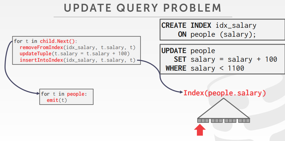
modification queries
- Operators that modify the database (INSERT, UPDATE, DELETE) are responsible for checking constraints and updating indexes
- UPDATE/DELETE:
- Child operators pass Record IDs for target tuples.
- Must keep track of previously seen tuples
- INSERT:
- Choice #1: Materialize tuples inside of the operator.
- Choice #2: Operator inserts any tuple passed in from child operators.
- 万圣节问题,更新tuple物理位置失败,导致scan的时候会看到tuple多次
- 最早在1976年 IBM System R研究人员发现的
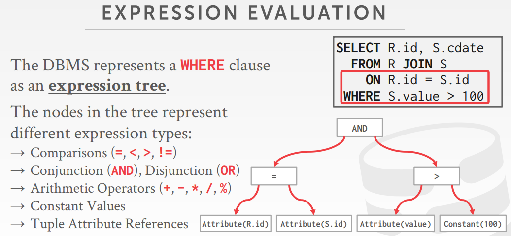
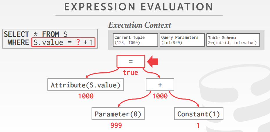
expression evaluation
Evaluating predicates in this manner is slow.
The DBMS traverses the tree and for each node that it visits it must figure out what the operator needs to do.
常量折叠
The same query plan can be executed in multiple different ways.
(Most) DBMSs will want to use index scans as much as possible.
Expression trees are flexible but slow
parallel vs distributed
- Parallel DBMSs
- Resources are physically close to each other.
- Resources communicate over high-speed interconnect.
- Communication is assumed to be cheap and reliable
- Distributed DBMSs
- Resources can be far from each other.
- Resources communicate using slow(er) interconnect.
- Communication cost and problems cannot be ignored
process models
- Process per DBMS Worker
- Each worker is a separate OS process.
- Relies on OS scheduler.
- Use shared-memory for global data structures.
- A process crash doesn’t take down entire system.
- Examples: IBM DB2, Postgres, Oracle
- Process Pool
- A worker uses any free process from the pool.
- Still relies on OS scheduler and shared memory.
- Bad for CPU cache locality.
- Examples: IBM DB2, Postgres (2015)
- Thread per DBMS Worker
- Single process with multiple worker threads.
- DBMS manages its own scheduling.
- May or may not use a dispatcher thread.
- Thread crash (may) kill the entire system.
- Examples: IBM DB2, MSSQL, MySQL, Oracle (2014)
- summary
- Advantages of a multi-threaded architecture:
- Less overhead per context switch.
- Do not have to manage shared memory.
- The thread per worker model does not mean that the DBMS supports intra-query parallelism.
scheduling
- For each query plan, the DBMS decides where, when, and how to execute it.
- How many tasks should it use?
- How many CPU cores should it use?
- What CPU core should the tasks execute on?
- Where should a task store its output?
- The DBMS always knows more than the OS.
parallelism
- Inter-Query,不同的查询之间是并行的
- 提升整体性能,降低延迟
- 如果都是只读的需要少量调度就可以,如果是更新则很难保证正确
- Intra-Query,单个查询内部是并行的
- 提升单个查询性能,可以使用生产者、消费者模式
- 使用多个线程访问中心数据结构、或者用分区隔离多个worker
- Use a separate worker to perform the join for each level of buckets for R and S after partitioning
intra-query parallelism
- Intra-Operator (Horizontal)
- Inter-Operator (Vertical)
- Bushy
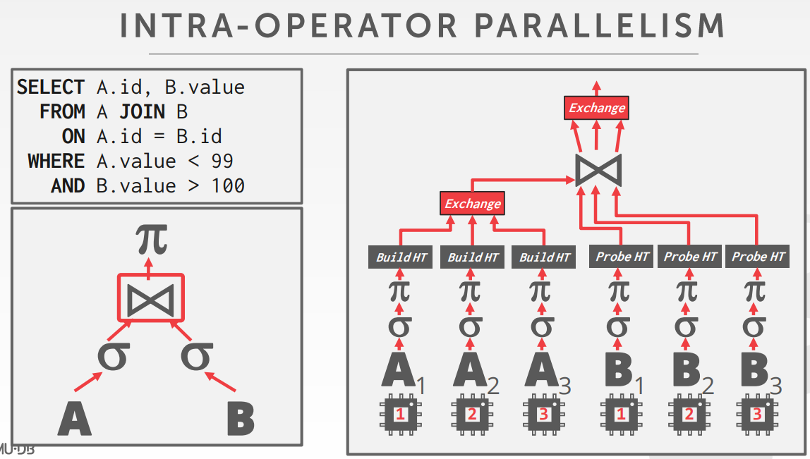
Intra-Operator (Horizontal)
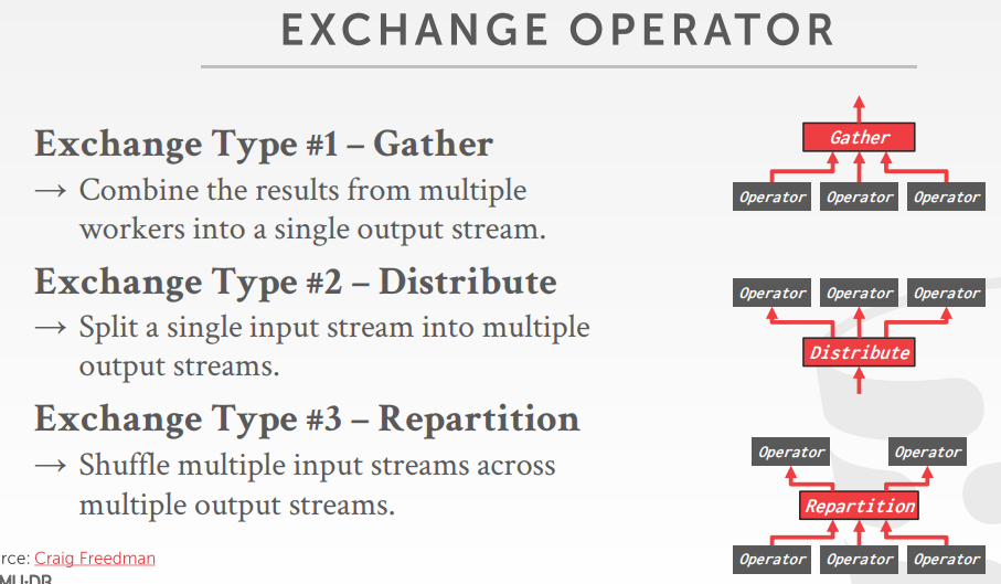
Decompose operators into independent fragments that perform the same function on different subsets of dataThe DBMS inserts an exchange operator into the query plan to coalesce/split results from multiple children/parent operators.
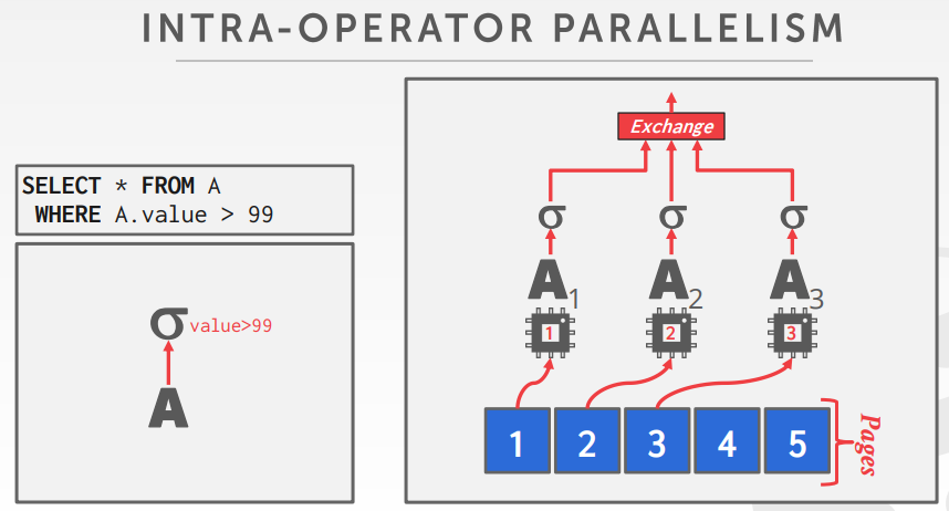
一个水平并行化的例子
|
|
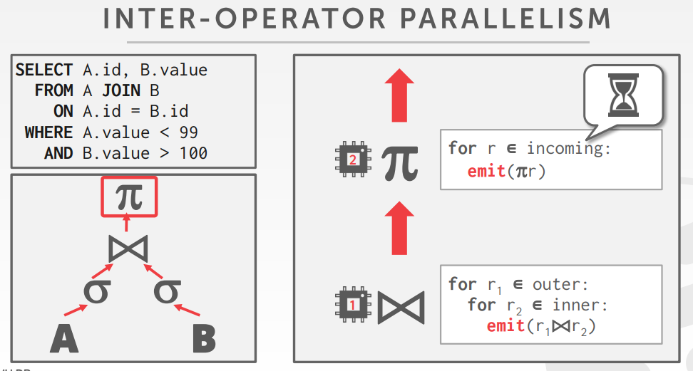
Inter-Operator (Vertical)
- Operations are overlapped in order to pipeline data from one stage to the next without materialization.
- Workers execute operators from different segments of a query plan at the same time.
- Also called pipeline parallelism.
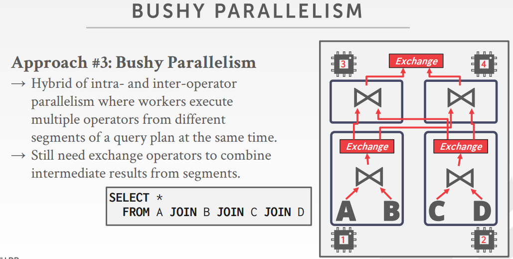
Bushy Parallelism
- Hybrid of intra- and inter-operator parallelism where workers execute multiple operators from different segments of a query plan at the same time.
- Still need exchange operators to combine intermediate results from segments.
Using additional processes/threads to execute queries in parallel won’t help if the disk is always the main bottleneck.
In fact, it can make things worse if each worker is working on different segments of the disk.
I/O parallelism
- Split the DBMS across multiple storage devices.
- Multiple Disks per Database
- One Database per Disk
- One Relation per Disk
- Split Relation across Multiple Disks
- 。。。
multi-disk parallelism
- Configure OS/hardware to store the DBMS’s files across multiple storage devices.
- Storage Appliances
- RAID Configuration, RAID 0、RAID 1
- This is transparent to the DBMS
database partition
- Some DBMSs allow you to specify the disk location of each individual database.
- The buffer pool manager maps a page to a disk location.
- This is also easy to do at the filesystem level if the DBMS stores each database in a separate directory.
- The DBMS recovery log file might still be shared if transactions can update multiple databases.
- Split single logical table into disjoint physical segments that are stored/managed separately.
- Partitioning should (ideally) be transparent to the application.
- The application should only access logical tables and not have to worry about how things are physically stored.
- vertical partition
- horizontal partition
- 水平分割方式:Hash Partitioning、Range Partitioning、Predicate Partitioning
Parallel execution is important, which is why (almost) every major DBMS supports it. However, it is hard t get right.
- Coordination Overhead
- Scheduling
- Concurrency Issues
- Resource Contention
相关文章
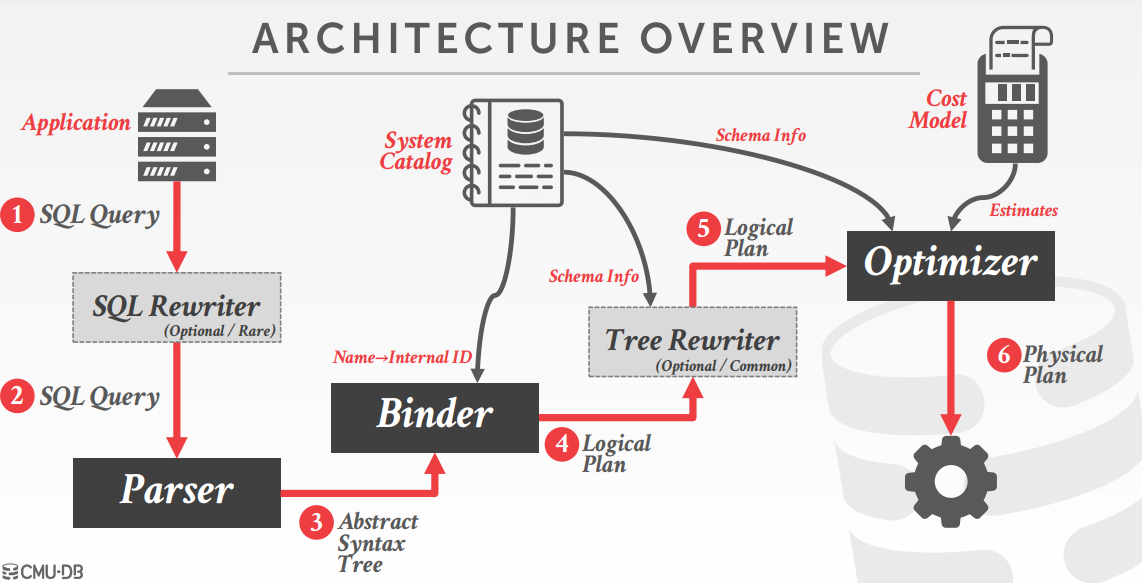
Query Planning & Optimization
Remember that SQL is declarative
User tells the DBMS what answer they want, not how to get the answer
There can be a big difference in performance based on plan is used
IBM System R
- First implementation of a query optimizer from the 1970s.
- People argued that the DBMS could never choose a query plan better than what a human could write.
- Many concepts and design decisions from the System R optimizer are still used today
query optimization
- Heuristics / Rules
- Rewrite the query to remove stupid / inefficient things.
- These techniques may need to examine catalog, but they do not need to examine data.
- Cost-based Search
- Use a model to estimate the cost of executing a plan
- Evaluate multiple equivalent plans for a query and pick the one with the lowest cost
logical VS physical plan
- The optimizer generates a mapping of a logical algebra expression to the optimal equivalent physical algebra expression
- Physical operators define a specific execution strategy using an access path.
- They can depend on the physical format of the data that they process (i.e., sorting, compression).
- Not always a 1:1 mapping from logical to physical.
query optimization is NP-hard
- This is the hardest part of building a DBMS
- If you are good at this, you will get paid $$$.
- People are starting to look at employing ML to improve the accuracy and efficacy of optimizers.
- IBM DB2 tried this with LEO in the early 2000s…
关系代数
- 如果生了相同的tuples,那么两个关系代数表达式是等价的
- DBMS可以识别出更好的查询几乎,而无需代价模型
- 这种也叫做查询重写
relational algebra equivalences
|
|
Joins:
- Commutative, associative
- R join S = S join R
- (R join S) join T = R join(S join T)
- The number of different join orderings for an nway join is a Catalan Number
- $O(4^n)$
projections
- 尽可能早的执行,这样数据量更少,中间结果也少
- 只输出必要的属性
- 对于列存不是很重要
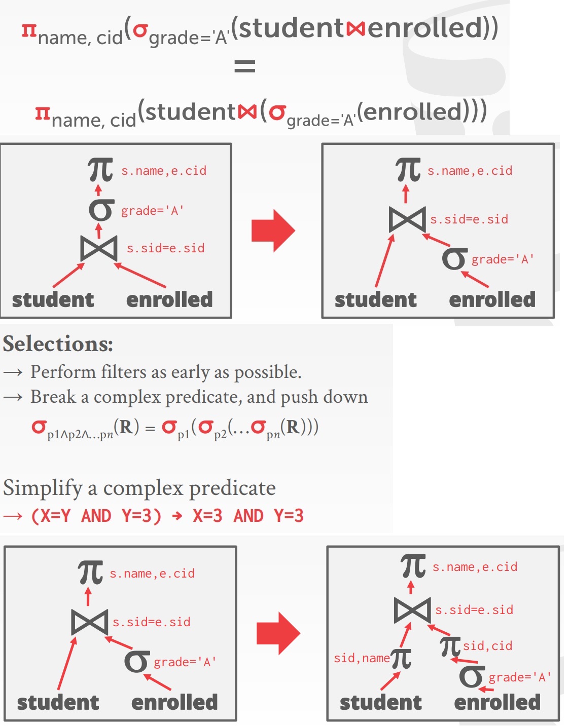
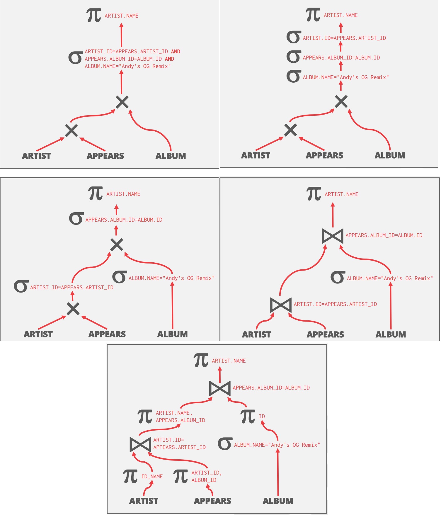
logical query optimization
- Transform a logical plan into an equivalent logical plan using pattern matching rules.
- The goal is to increase the likelihood of enumerating the optimal plan in the search.
- Cannot compare plans because there is no cost model but can “direct” a transformation to a preferred side.
- Split Conjunctive Predicates,Decompose predicates into their simplest forms to make it easier for the optimizer to move them around.
- Predicate Pushdown,Move the predicate to the lowest applicable point in the plan.
- Replace Cartesian Products with Joins,Replace all Cartesian Products with inner joins using the join predicates.
- Projection Pushdown,Eliminate redundant attributes before pipeline breakers to reduce materialization cost
nested sub-queries
- The DBMS treats nested sub-queries in the where clause as functions that take parameters and return a single value or set of values.
- Rewrite to de-correlate and/or flatten them
- Decompose nested query and store result to temporary table
子查询重写的例子:
|
|
分解查询
|
|
expression rewriting
- An optimizer transforms a query’s expressions (e.g., WHERE clause predicates) into the optimal/minimal set of expressions.
- Implemented using if/then/else clauses or a pattern-matching rule engine.
- Search for expressions that match a pattern.
- When a match is found, rewrite the expression.
- Halt if there are no more rules that match.
more example
|
|
cost model componets
- Physical Costs
- Predict CPU cycles, I/O, cache misses, RAM consumption, pre-fetching, etc…
- Depends heavily on hardware
- Logical Costs
- Estimate result sizes per operator.
- Independent of the operator algorithm.
- Need estimations for operator result sizes
- Algorithmic Costs
- Complexity of the operator algorithm implementation
disk-based DBMS cost model
- The number of disk accesses will always dominate the execution time of a query.
- CPU costs are negligible.
- Must consider sequential vs. random I/O.
- This is easier to model if the DBMS has full control over buffer management.
- We will know the replacement strategy, pinning, and assume exclusive access to disk
- PG cost model,结合了CPU和I/O cast,增加了magic的常量的权重
- 默认设置是面向磁盘的,但对于大内存不合适
- 读tuple内存是磁盘的400x,顺序I/O是随机的4x
- IBM DB2 cost,考虑的硬件环境、存储设备、通讯带宽、内存资源
- 并发环境:平均用户数、隔离级别、阻塞情况、可用的lock数量
不同数据的优化命令
- Postgres/SQLite: ANALYZE
- Oracle/MySQL: ANALYZE TABLE
- SQL Server: UPDATE STATISTICS
- DB2: RUNSTATS
统计信息
- 对于每个关系R,Nr R的tuple数量
- V(A,R),属性A 不同value的数量
- selection cardinality SC(A,R),属性A值的平均记录数据, Nr / V(A,R)
- 这个公式假定了所有数据出现的频率是一样的
- 等值条件如id=123这种评估比较简单
- 复杂度val>100,age=30 and status=‘aa’ and age+id in(1,2,3) 这种评估就困难了
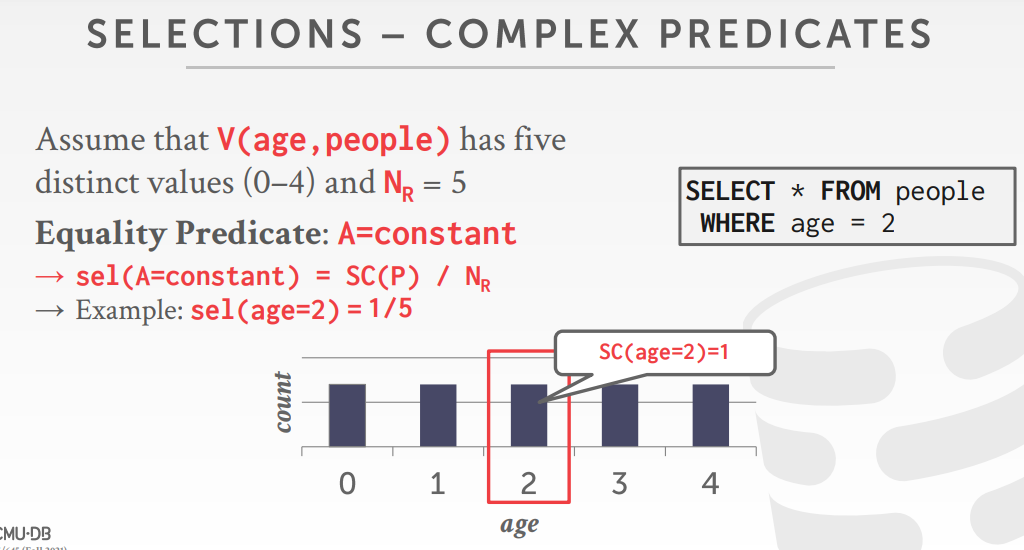
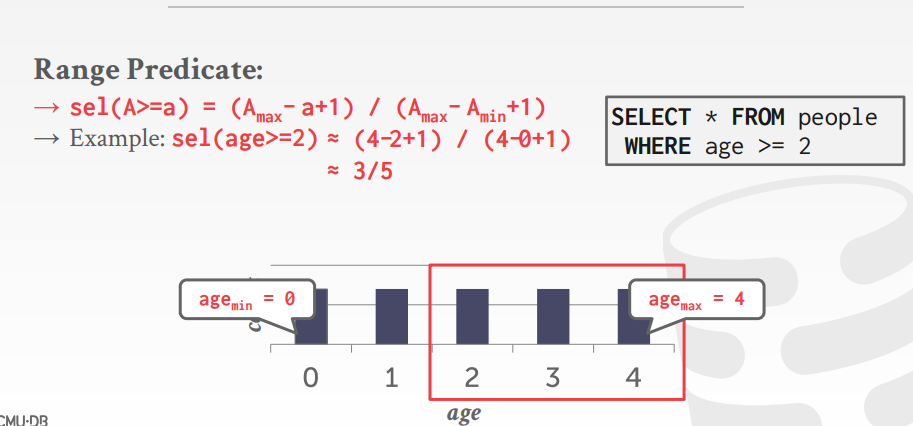
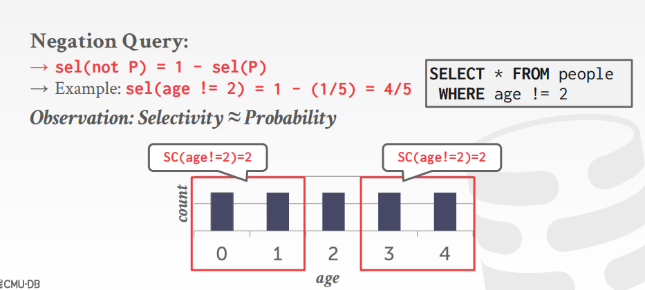
复杂的谓词
- The selectivity (sel) of a predicate P is the fraction of tuples that qualify
- 公式依赖下面类型谓词
- Equality
- Range
- Negation
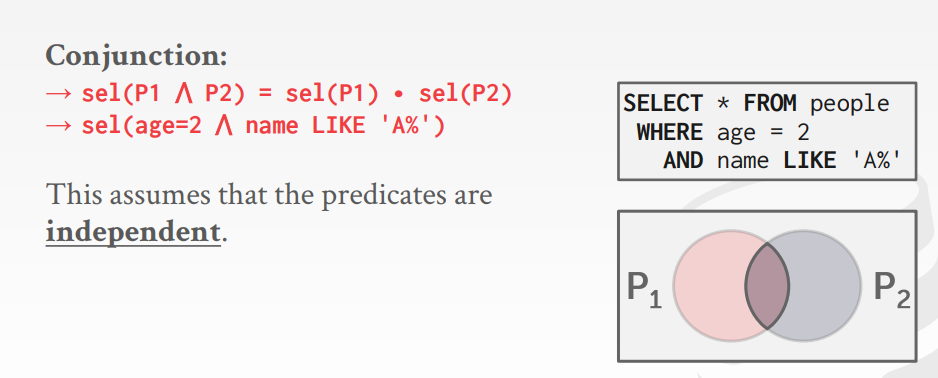
- Conjunction
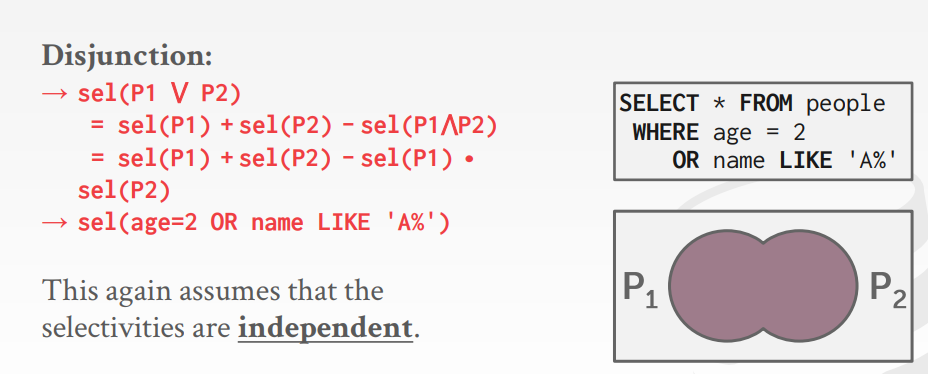
- Disjunction
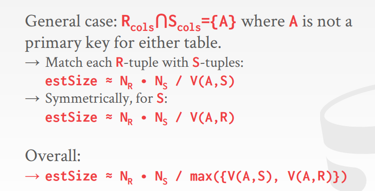
result size estimation for joins
选择基础 selection cardinality
- 假设:
- Uniform Data
- The distribution of values (except for the heavy hitters) is the same.
- Independent Predicates
- The predicates on attributes are independent
- Inclusion Principle
- The domain of join keys overlap such that each key in the inner relation will also exist in the outer table
基于概率的选择
- where customer.balance < 1000 and orders.total > 10000
- 找到customer筛选后小,还是orders筛选后数量小
- 数据分布可能不是均匀的
- 等宽直方图,All buckets have the same width (i.e., the same number of values)
- 等高直方图,Vary the width of buckets so that the total number of occurrences for each bucket is roughly the same
- Probabilistic data structures that generate approximate statistics about a data set.
- Cost-model can replace histograms with sketches to improve its selectivity estimate accuracy
- Count-Min Sketch (1988): Approximate frequency count of elements in a set.
- HyperLogLog (2007): Approximate the number of distinct elements in a set
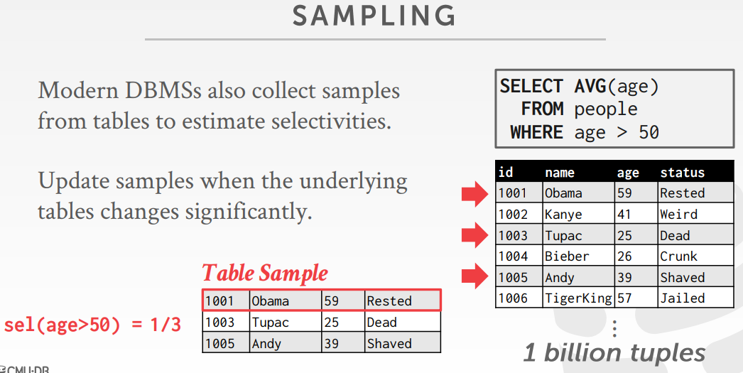
sampling
查询优化
- RBO重新plan之后,就需要枚举所有的plan然后评估他们的cost
- Single relation.
- Multiple relations.
- Nested sub-queries
- It chooses the best plan it has seen for the query after exhausting all plans or some timeout
single-relation query planning
- Sequential Scan
- Binary Search (clustered indexes)
- Index Scan
- 主要是OLTP场景,用启发式搜索就足够了,因为都比较简单
- Joins are almost always on foreign key relationships with a small cardinality
multi-relation query planning
- 随着JOIN数量的增长,查询的时间复杂度也急剧增长,需要限制搜索空间
- IBM Sytem R,限制了 left-deep-join
- 如果要考虑到 bushy tree,那么搜索空间太多了,所以放弃,但是bushy tree适合join并发执行
- left-deep-join像流水线一样执行
- 枚举所有顺序:left-deep tree#1, left-deep-tree#2, #3 …
- 枚举所有的算子:hash join, sore-merge join, nsted loop join
- 枚举所有的访问范式: index#1, index#2, seq scan …
- Use dynamic programming to reduce the number of cost estimations
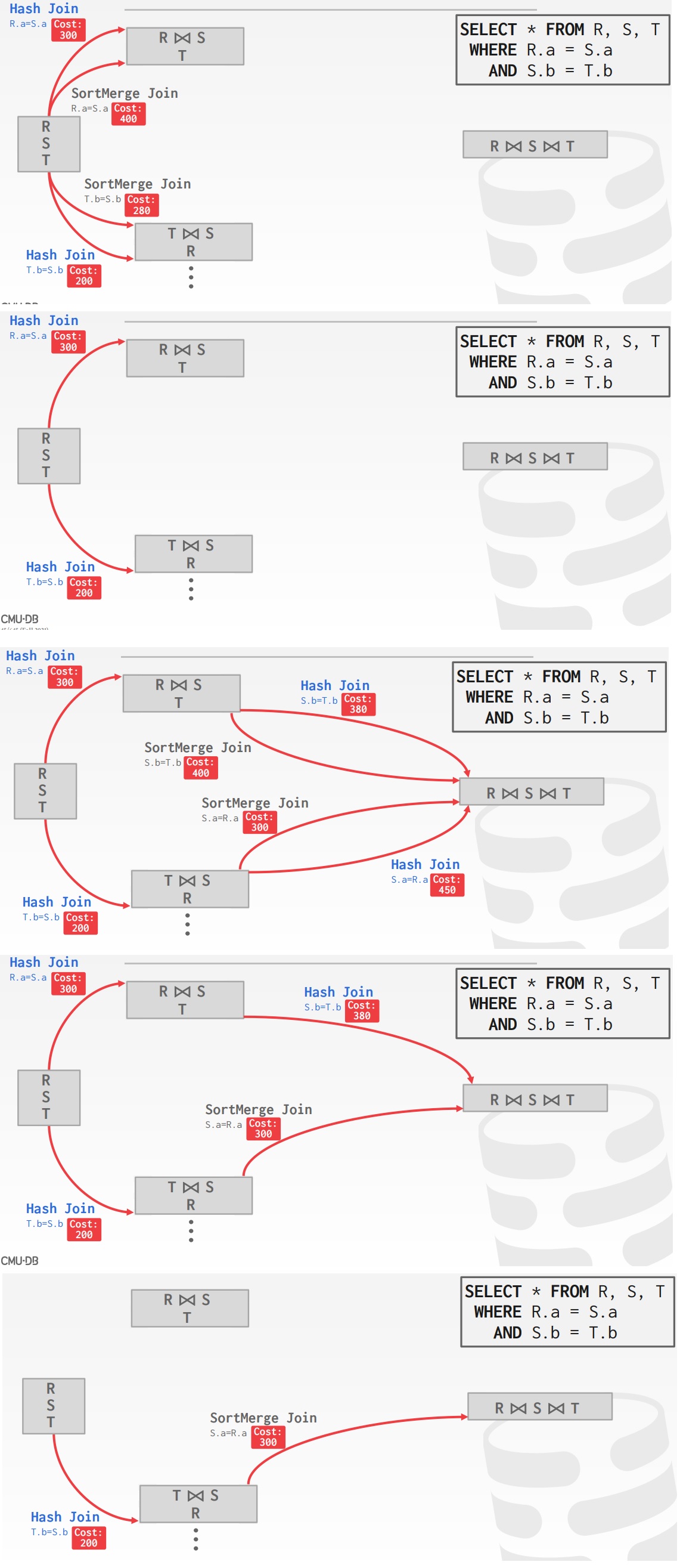
动态规划的执行方式,假设有如下SQL
|
|
执行过程:
- 计算 R join S的hash join,sort-merge join成本,计算T join S的两个join成本
- 对比发现,R join S用hash join最低
- T join S 用hash join最低
- 计算R join S join T的两个join成本,计算 T join S join R的两个join成本
- 找到上述最低的成本
- 自后确定全局最低的成本join方式
candidate plan example,注意真实的数据库并不是这样执行的
|
|

postgrs 优化器
- Examines all types of join trees
- Left-deep, Right-deep, bushy
- Two optimizer implementations:
- Traditional Dynamic Programming Approach
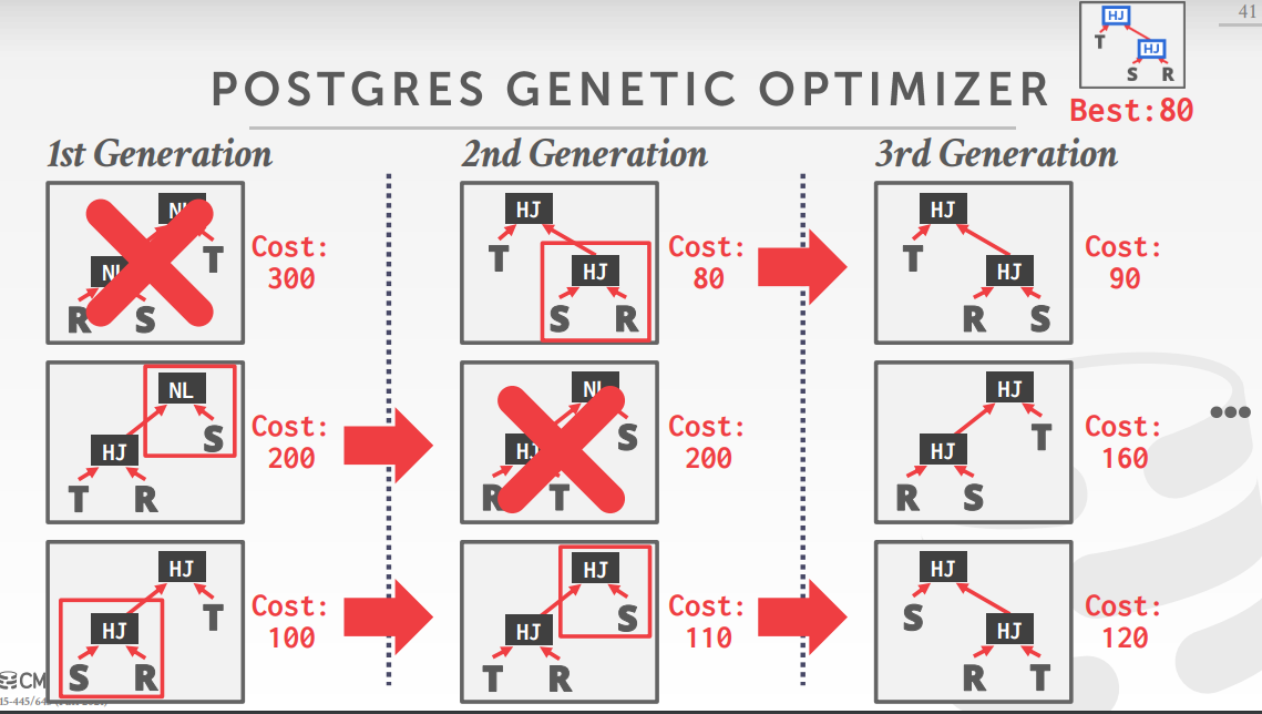
- Genetic Query Optimizer (GEQO)
- 当tables < 12时,用传统的 动态规划,如果>=12,则使用 遗传查询优化
相关文章
- LEO: An autonomic query optimizer for DB2
- Catalan_number
- PostgreSQL Query Planning
- Query Optimization
- 10 Cool SQL Optimisations That do not Depend on the Cost Model
- Count-Min Sketch
- HyperLogLog
- MyQL 直方图
- IS QUERY OPTIMIZATION A “SOLVED” PROBLEM?
- Genetic Query Optimization (GEQO) in PostgreSQL
- PostgreSQL 中的遗传查询优化(GEQO)