原文
https://15721.courses.cs.cmu.edu/spring2023/papers/09-compilation/p539-neumann.pdf
背景
数据库一般将查询 转换为物理代数中的表达式,然后计算这个代数表达式并产生 查询结果
传统方式是通过Volcano-style模型来实现的,每个物理算子都会产生一个tuple返回给其输入(父节点),然后父节点反复调用next函数,不停的获取这个tuple流
这种设计非常清晰,也非常容易扩展,可以支持任意的算子
对于I/O为主的数据库来说比较合适,因为CPU不是瓶颈
- 每次next函数只会返回一个tuple(当做中间结果/最终结果),这也消耗了不少时间
- 虚函数调用比普通函数调用更耗时,对现代CPU来说导致分支预测下降
- 这种模式对于数据本地性来说不好,而且需要复杂的维护机制
改进方式也很简单,每次返回一批tuple就可以了
不过这样也违背了数据流的特点,必须将数据保存、物化,父节点才能访问,也消耗了一些带宽
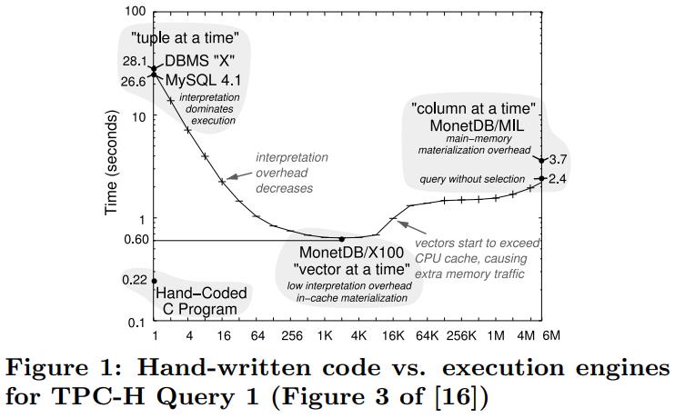
从手写代码来看,其效率比迭代模式、全量物化模式,以及MonetDB/X100 的向量化模式更好(向量化也达不到手写的性能)
由于聚合查询的结果是唯一的,因此执行不好的都属于次优实现
HIQUE的生成了C源码然后编译,在算子执行期间执行inline物化结果,来消除迭代模型
其他一些优化包括
- 使用SIMD来优化独立表达式
- 组合连接的谓词,这需要在分支数量 和 评估谓词数量 之间做权衡
论文实现了一个新的查询编译策略
- 以数据为中心,而不是操作为中心,处理尽可能长的保持在CPU寄存器中,算子的边界变得模糊
- 采用push方式,而不是pull方式,这样有更好的数据本地性
- 查询编译为原生的机器代码,这里使用的是LLVM编译框架
这里生成的不是 C、或者C++源码,而是LLVM字节码,后面可以实现更多的优化技巧,而高级语言如C++ 就不好实现
由于是依靠编译器的,所以当编译器升级了,优化也就自动升级了,而非编译方式的系统,需要手动更新优化模块
实现
这里定义两个概念
- pipeline breaker,如果流入的数据超出了CPU寄存器
- full pipeline breaker,在继续处理之前,物化了所有来自这一端的输入tuple
所谓断开,就是寄存器、cache放不下,需要溢出到内存了,这样做的目的是尽可能长的,让数据保留在cache中
火山模型需要有大量调用,每次调用相当于断开管道,都会刷新寄存器
批模型减少了调用次数,但产生的tuple太多,也会断开管道
实际上,任何 迭代风格使用的是pull模型,都有断开管道的风险,但有时候产生的tuple数量很少,并不需要拷贝
Query Processing Architecture
论文中采用的是 push模型,数据总是从 一个 pipeline-breaker push到另一个 pipeline-breaker
以一个SQL为例,三个表的join,其中R2是一个子查询,做了group by
R2会跟R3做join,其结果再跟R1做join
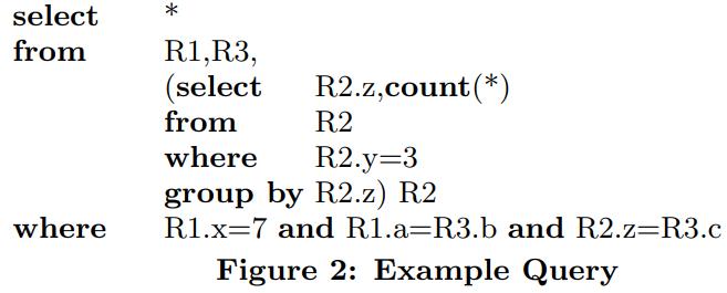
传统的方式,比如根节点需要输出(a=b)的join结果,那么会先去左边建立hash表(递归的执行),然后再去右边节点去探测
这样的话效率不好
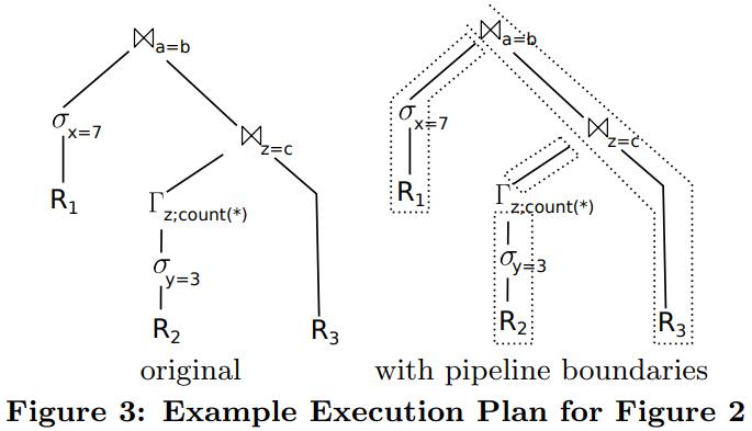
论文中提出将整个执行过程分成了 4个部分,也就是 4个管道,在管道内部可以最大化CPU利用率,管道之间通过物化方式传递
下图是整个执行的伪代码,代码中包含了 4个片段,就对应 4个管道
- 管道1,filter R1,将结果放入hash 表 (a,b)中
- 管道2,类似的遍历R2将结果放入Γz 中
- 管道3,将Γz 的结果写入到 hash表 (z=c)中
- 管道4,遍历R3,沿着对应的几个hash表,并产出结果
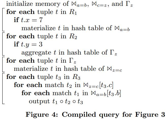
这些循环保证了 很好的代码本地行,其性能也大大超过了迭代模型
Compiling Algebraic Expressions
code-gen非常不同于迭代模式,它没有什么规则,其左边的解构 跟右边的完全不同
从编译器的视角看,每个算子都有两个操作
- produce()
- consume(attributes, source)
通过调用 produce 函数,对应的算子产生它的结果,然后将其push到 consume算子(通过调用consume函数)
对于figure3,其执行过程如下:
- 查询首先调用 (a=b)produce,用来填充hash表
- 这个produce又会调用 σx=7,这会触发R1的produce
- R1这个produce是叶节点,然后产生tuple,这就会调用到 σx=7 来做消费
- σx=7 消费是通过选择某个固定的投影,满足的结果会传递给(a=b)
- 这样最上面的那个join的左边就完成了,将其存储到hash表中
- 之后控制流重新回到join,它会再调用 (c=z)来对右边的结果做probe
produce、consume只是一个概念的模型,只是用于代码生成的时候会使用到
SQL执行还是跟往常一样,只是到了生成物理执行计划时,这步被替代了,使用code-gen生成了一段代码
code-gen使用produce、consume模型来生成最终的代码
使用figure5中的规则,应用到 figure3,就能产生出 figure4的伪代码了
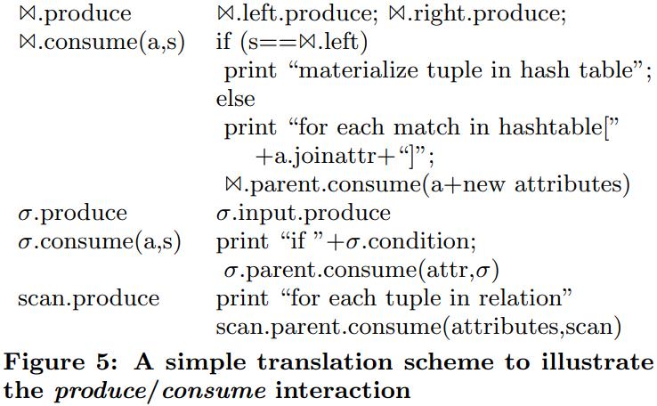 真实的场景自然比这个要复杂很多,包括跟踪加载的属性、牵涉到算子状态、相关子查询中的属性依赖等
代码生成
Generating Machine Code
最初code-gen是生成了C++代码,但这需要编译C++代码
- 一个复杂的编译+优化 可能要好几秒
- C++不提供对生成代码的控制,这可能会导致性能不佳
论文中使用了 Low Level Virtual Machine (LLVM)
- 它可以生成跨平台的汇编代码
- 之后由LLVM提供的优化的JIT编译器直接执行
LLVM
- 并不是完全的汇编代码,而更像是偏底层的中间代码
- 它隐藏了寄存器分配问题,可以提供无限多的寄存器
- LLVM汇编代码是可以跨平台的,会由LLVM JIT来生成具体平台的机器代码
- 其代码是强类型的,这样可以发现很多C++代码中的一些bug
- 优化能力很强,编译速度非常快:几微秒;而C++编译器可能需要几秒
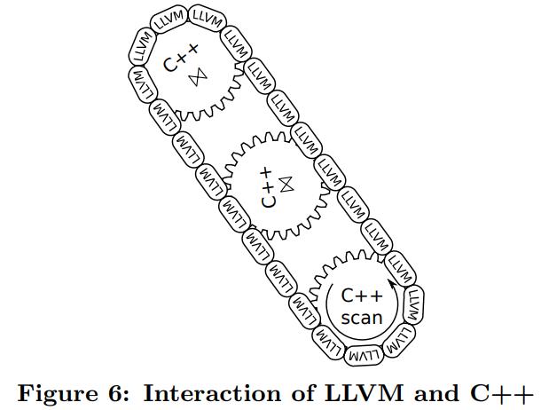
不是所有的查询操作都是LLVM代码,这样的化编写起来很麻烦,只有一些复杂的操作是用C++写的
之后用LLVM把C++代码,和LLVM汇编代码链接起来
比如:scan部分,这里需要加载复杂的结构,找出next,就是用C++写的
这部分的逻辑会驱动执行流水线,后面的tuple的自身访问、以及filter、物化到hash表中都是LLVM汇编
C++和LLVM汇编是交互执行的,比如sort操作会返回到C++部分,一旦操作完了LLVM汇编就会直接操作这些数据块了
大部分时间都是LLVM工作,而且都是cache和寄存器交互的,所以执行很快
Complex Operators
将复杂的查询编译为单个函数是不可能的、不可取的
- LLVM代码可能在某时调用C++代码接管控制流,比如初始的外排序由LLVM做,控制合并阶段由C++做,根据需要调用LLVM代码
- 将整个查询逻辑完全inline到一个函数,可能会导致代码量指数增长
- 比如join的inner部分可能调用consume这时候有两个结果,匹配或者不匹配,而这两种结果又会级联调用outer,这就导致了代码指数增长
- 所以更好的方式是,确保热点部分不要跨函数调用,统一放到LLVM代码里面
因篇幅有限这里只展示部分的LLVM代码,也就是scan R2那段的逻辑
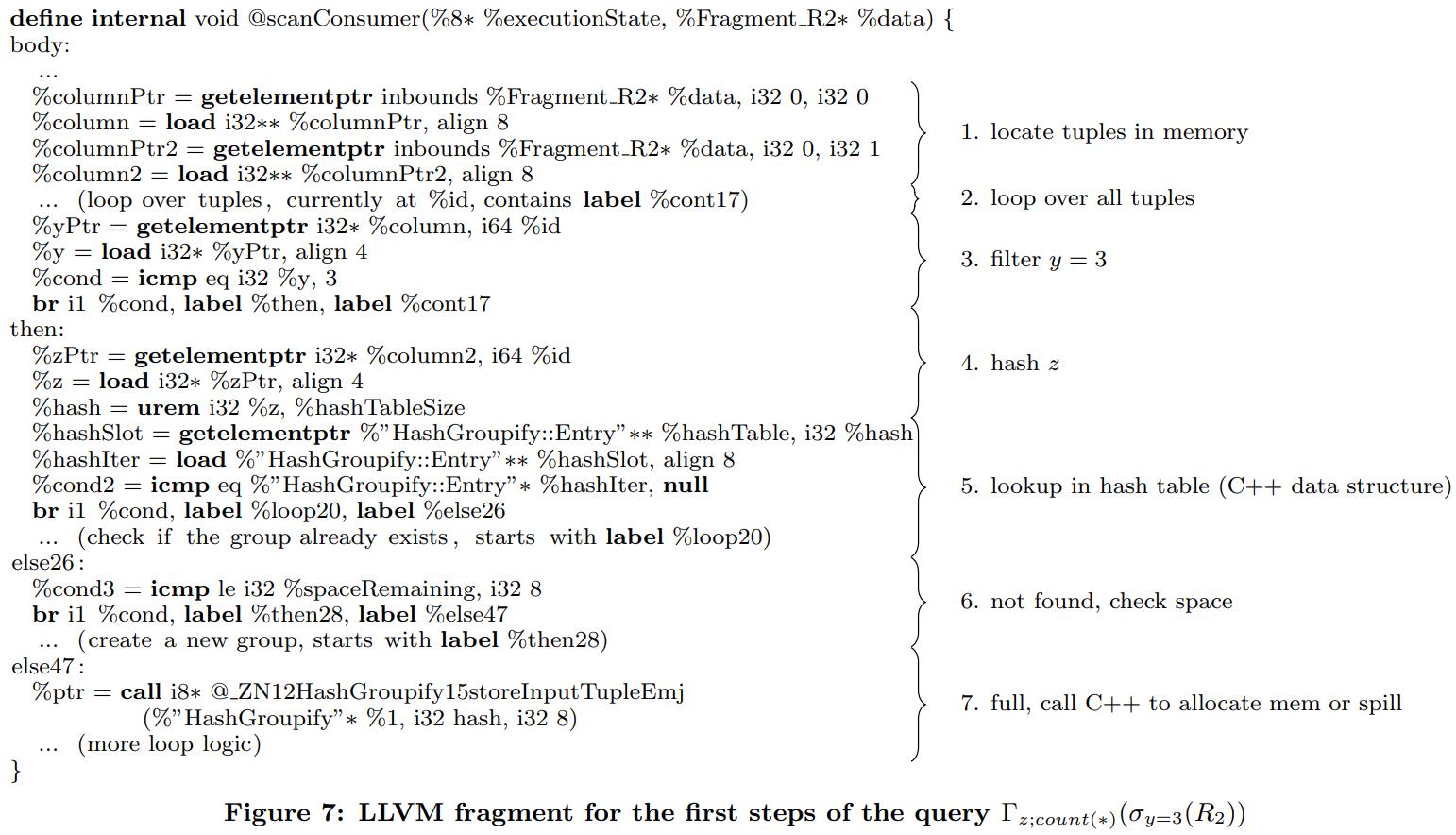
主要逻辑
- LLVM代码首先load需要的列
- 然后loop所有的tuple,再加载属性 y 放到寄存器中
- 如果不满足谓词则继续loop
- 如果满足则是then分支,读取属性 z到寄存器计算hash值,使用hash值去hash表中查找(这里使用了C++的数据结构)
- 如果没找到匹配的组,检查是否有足够空间分配新的组,没有则调用C++函数分配新空间,如果需要的话会溢出到内存
- 主要的热点代码都是由LLVM完成的,核心逻辑都是在 then块内
- 注意这里的LLVM是直接调用了C++代码,所以C++和LLVM代码可以相互直接调用,没有性能损失
以TPC-H为例,Query-1是一个单表查询,只有基于hash的聚合,但论文发现,初始化时有50%的时间花在了hash上了
另一个花费比较大的是分支
- 如果一个分支总是返回true、或者false,那就表现的不错
- 但是如果已50%的概率返回结果,那么会对性能有很大影响
比如下面这段就不是分支友好的
1
2
3
4
5
|
Entry* iter=hashTable[hash];
while (iter) {
	... // inspect the entry
	iter=iter->next;
}
|
上面的代码不好的原因while是混合了两件事
- 检查指定的hash值是否存在
- 检查是否达到了链表末尾
上述第一次检查的时候几乎总是 true(假设hash表被填充了)
而第二次检查总是为false(hash碰撞的list很短)
下面是分支友好的
1
2
3
4
5
|
Entry* iter=hashTable[hash];
if (iter) do {
	... // inspect the entry
	iter=iter->next;
} while (iter);
|
上面这个小改动,对于hash表探测提升了20%的性能
高级并行化技术
目前处理的方式都是一次一个tuple,基本都是线性的
但我们还是可以整合其他更先进的技术
传统方式使用块来访问并不是很好,因为需要多的内存访问,但如果将块发能放入寄存器中则非常好
也就是使用SIMD技术
- 首先使用利用现代CPU巨大的加速
- 其次,可以缓解分支问题
LLVM支持SIMD技术,允许将值当做向量处理
现代CPU都是多核的,所以DBMS如何利用多核加速就很重要了
比如对输入数据做分区,然后合并,就可以并行化
而LLVM的存在,使得figure-7这样的代码块能更好的支持并行化
因为他们本身都是一个一个的片段,片段内都是紧耦合的,能很好的并行化处理
五个查询在 论文的附录D 中,这里就不贴了
OLTP使用了单线程查询,OLAP也是另外不做更新
对比了Hpyer的原始版本、code-gen版本、MonetDB、以及一个商业数据库
LOTP
评估
由于存储系统对查询性能影响很大,这里分成两部分
- 完整的系统比较,包括代码生成的分析
- 基准测试,用于测试特定算子行为
Systems Comparison
目前这个技术已经整合到Hpyer中了,可以混合OLAP和OLTP
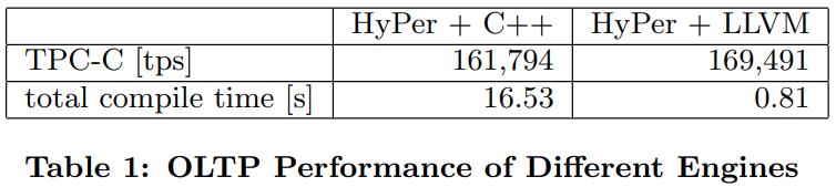
使用的是 TPC-CH测试集,对于OLTP的使用TPC-C,对于OLAP的使用TPC-H
OLTP对比如下,TPC来看,C++版本和code-gen差不多,code-gen略好一点
但是编译时间看,code-gen只需要 十分之一的时间
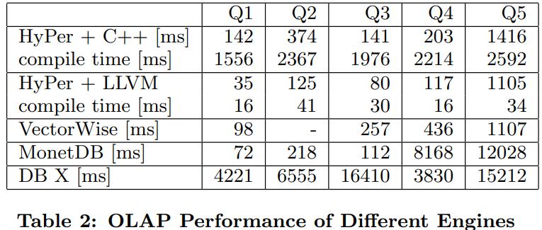
下面是OLAP的比较,DB X是面向磁盘的所以比较慢,不过执行的数据集已经能放入内存了
除了DB X其他几个执行时间都挺快
HyPer的C++编译时间太长了,都超过了执行时间,这也是需要替换的原因
Code Quality
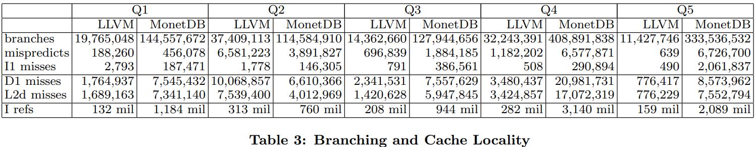
使用callgrind工具(来自valgrind)分析 5个查询
是用来分析分支和缓存有效性
下面是和 MonetDB的对比,除了Q2,其他的分支以及预测失败都比MonetDB少很多
D1的miss、L2miss也是比MonetDB少很多(除了Q2)
最后是生成的指令,也是比MonetDB少很多
附录
OPERATOR TRANSLATION
Scan
使用 ScanConsumer 辅助类来访问所有相关的片段,访问的所有tuple都包含在当前的片段中
在需要的时候注册可用的列,传递tuple到消费算子
跟关系类型的不同,ScanConsumer可能会创建对C++函数的调研
由于scan是叶子节点算子,它没有consume部分
 1
 2
 3
 4
 5
 6
 7
 8
 9
10
11
12
13
14
15
16
17
18
19
20
21
22
23
24
25
26
27
28
29
30
31
32
33
34
35
36
37
38
39
|
void TableScanTranslator::produce(CodeGen& codegen,Context& context) const {
	// Access all relation fragments
	llvm::Value∗ dbPtr=codegen.getDatabasePointer();
	llvm::Value∗ relationPtr=codegen.getPtr(dbPtr,db.layout.relations[table]);
	auto& required=scanConsumer.getPartitionPtr();
	ScanConsumer scanConsumer(codegen,context)
	for (;db.relations[table]−>generateScan(codegen,relationPtr,scanConsumer);) {
		// Prepare accessing the current fragment
		llvm::Value∗ partitionPtr=required;
		ColumnAccess columnAccess(partitionPtr,required);

		// Loop over all tuples
		llvm::Value∗ tid=codegen.const64(0);
		llvm::Value∗ limit=codegen.load(partitionPtr,getLayout().size);
		Loop loop(codegen,codegen−>CreateICmpULT(tid,limit),{{tid,”tid”}}); {
			tid=loop.getLoopVar(0);

			// Prepare column access code
			PartitionAccess::ColumnAccess::Row rowAccess(columnAccess,tid);
			vector<ValueAccess> access;
			for (auto iter=required.begin(),limit=required.end();iter!=limit;++iter)
				access.push back(rowAccess.loadAttribute(∗iter));

				// Register providers in new inner context
				ConsumerContext consumerContext(context);
				unsigned slot=0;
				for (auto iter=required.begin(),limit=required.end();iter!=limit;++iter,++slot)
					consumerContext.registerIUProvider(&(getOutput()[∗iter].iu),&access[slot]);

					// Push results to consuming operators
					getParent()−>consume(codegen,consumerContext);

					// Go to the next tuple
					tid=codegen−>CreateAdd(tid,codegen.const64(1));
					loop.loopDone(codegen−>CreateICmpULT(tid,limit),{tid});
			}
		}
	}
}
|
Selection
这里的produce部分很简单,增加需要的属性到谓词上下文中,然后调用输入端的produce
consume部分会filter做过滤
 1
 2
 3
 4
 5
 6
 7
 8
 9
10
11
12
13
14
15
|
void SelectTranslator::produce(CodeGen& codegen,Context& context) const {
	// Ask the input operator to produce tuples
	AddRequired addRequired(context,getCondition().getUsed());
	input−>produce(codegen,context);
}

void SelectTranslator::consume(CodeGen& codegen,Context& context) const {
	// Evaluate the predicate
	ResultValue value=codegen.deriveValue(getCondition(),context);

	// Pass tuple to parent if the predicate is satisfied
	CodeGen::If checkCond(codegen,value); {
		getParent()−>consume(codegen,context);
	}
}
|
Projection
更简单,其consume部分是空的,直接调用其父节点
 1
 2
 3
 4
 5
 6
 7
 8
 9
10
|
void ProjectTranslator::produce(CodeGen& codegen,Context& context) const {
	// Ask the input operator to produce tuples
	SetRequired setRequired(context,getOutput());
	input−>produce(codegen,context);
}

void ProjectTranslator::consume(CodeGen& codegen,Context& context) const {
	// No code required here, pass to parent
	getParent()−>consume(codegen,context);
}
|
Map
map操作符通过求值函数计算新列
计算的位置,映射和选择已经由优化器完成了
 1
 2
 3
 4
 5
 6
 7
 8
 9
10
11
12
13
14
15
16
17
18
19
20
21
22
23
24
|
void MapTranslator::produce(CodeGen& codegen,Context& context) const {
	// Figure out which columns have to be provided by the input operator
	IUSet required=context.getRequired();
	for (auto iter=functions.begin(),limit=functions.end();iter!=limit;++iter) {
		(*iter).function−>getUsed(required);
		required.erase((∗iter).result);
	}

	// Ask the input operator to produce tuples
	SetRequired setRequired(context,required);
	input−>produce(codegen,context);
}

void MapTranslator::consume(CodeGen& codegen,Context& context) const {
	// Offer new columns
	vector<ExpressionAccess> accessors;
	for (auto iter=functions.begin(),limit=functions.end();iter!=limit;++iter)
		accessors.push back(ExpressionAccess(codegen,∗(∗iter).function));
	for (unsigned index=0,limit=accessors.size();index<limit;index++)
		context.registerIUProvider(functions[index].result,&accessors[index]);

	// Pass to parent
	getParent()−>consume(codegen,context);
}
|
Hash Join
这部分就很复杂了,LLVM的代码控制流会转回C++
首先会build hash部分,如果需要会溢出到磁盘,如果内存足够就会调用probe部分
如果左边build溢出了,则probe部分也要溢出
为了简化这里限制为inner join
 1
 2
 3
 4
 5
 6
 7
 8
 9
10
11
12
13
14
15
16
17
18
19
20
21
22
23
24
25
26
27
28
29
30
31
32
33
34
35
36
37
38
39
40
41
42
43
44
45
46
|
void HashJoin::Inner::produce() {
	// Read the build side
	initMem();
	produceLeft();
	if (inMem) {
		buildHashTable();
	} else {
		// Spool remaining tuples to disk
		spoolLeft();
		finishSpoolLeft();
	}

	// Is a in−memory join possible?
	if (inMem) {
		produceRight();
		return;
	}

	// No, spool the right hand side, too
	spoolRight();
	// Grace hash join
	loadPartition(0);
	while (true) {
		// More tuples on the right?
		for (;rightScanRemaining;) {
			const void∗ rightTuple=nextRight();
			for (LookupHash lookup(rightTuple);lookup;++lookup) {
				join(lookup.data(),rightTuple);
			}
		}

		// Handle overflow in n:m case
		if (overflow) {
			loadPartitionLeft();
			resetRightScan();
			continue;
		}

		// Go to the next partition
		if ((++inMemPartition)>=partitionCount) {
			return;
		} else {
			loadPartition(inMemPartition);
		}
	}
}
|
这里包含了三个函数,produce、consume、join
当溢出到磁盘时,可以直接调用 join函数
hash表已经在C++中实现了,所以join只可能在连接候选条件的时候调用
produce将控制流转回给C++,
consume部分确定相关的寄存器,并将他们物化到hash-table中
 1
 2
 3
 4
 5
 6
 7
 8
 9
10
11
12
13
14
15
16
17
18
19
20
21
22
23
24
25
26
27
28
29
30
31
32
33
34
35
36
37
38
39
40
41
42
43
44
45
46
47
48
49
50
51
52
53
54
55
56
57
58
59
60
61
62
63
64
65
66
67
68
|
void HJTranslatorInner::produce(CodeGen& codegen,Context& context) const {
	// Construct functions that will be be called from the C++ code
	{
		AddRequired addRequired(context,getCondiution().getUsed().limitTo(left));
		produceLeft=codegen.derivePlanFunction(left,context);
	}
	{
		AddRequired addRequired(context,getCondiution().getUsed().limitTo(right));
		produceRight=codegen.derivePlanFunction(right,context);
	}
	// Call the C++ code
	codegen.call(HashJoinInnerProxy::produce.getFunction(codegen),
		{context.getOperator(this)});
}

void HJTranslatorInner::consume(CodeGen& codegen,Context& context) const {
	llvm::Value∗ opPtr=context.getOperator(this);

	// Left side
	if (source==left) {
		// Collect registers from the left side
		vector<ResultValue> materializedValues;
		matHelperLeft.collectValues(codegen,context,materializedValues);

		// Compute size and hash value
		llvm::Value∗ size=matHelperLeft.computeSize(codegen,materializedValues);
		llvm::Value∗ hash=matHelperLeft.computeHash(codegen,materializedValues);
		// Materialize in hash table, spools to disk if needed
		llvm::Value∗ ptr=codegen.callBase(HashJoinProxy::storeLeftInputTuple,
		{opPtr,size,hash});
		matHelperLeft.materialize(codegen,ptr,materializedValues);

	// Right side
	} else {
		// Collect registers from the right side
		vector<ResultValue> materializedValues;
		matHelperRight.collectValues(codegen,context,materializedValues);

		// Compute size and hash value
		llvm::Value∗ size=matHelperRight.computeSize(codegen,materializedValues);
		llvm::Value∗ hash=matHelperRight.computeHash(codegen,materializedValues);

		// Materialize in memory, spools to disk if needed, implicitly joins
		llvm::Value∗ ptr=codegen.callBase(HashJoinProxy::storeRightInputTuple, {opPtr,size});
		matHelperRight.materialize(codegen,ptr,materializedValues);
		codegen.call(HashJoinInnerProxy::storeRightInputTupleDone,{opPtr,hash});
	}
}

void HJTranslatorInner::join(CodeGen& codegen,Context& context) const {
	llvm::Value∗ leftPtr=context.getLeftTuple(),∗rightPtr=context.getLeftTuple();
	// Load into registers. Actual load may be delayed by optimizer
	vector<ResultValue> leftValues,rightValues;
	matHelperLeft.dematerialize(codegen,leftPtr,leftValues,context);
	matHelperRight.dematerialize(codegen,rightPtr,rightValues,context);

	// Check the join condition, return false for mismatches
	llvm::BasicBlock∗ returnFalseBB=constructReturnFalseBB(codegen);
	MaterializationHelper::testValues(codegen,leftValues,rightValues,
		joinPredicateIs,returnFalseBB);
	for (auto iter=residuals.begin(),limit=residuals.end();iter!=limit;++iter) {
		ResultValue v=codegen.deriveValue(∗∗iter,context);
		CodeGen::If checkCondition(codegen,v,0,returnFalseBB);
	}

	// Found a match, propagate up
	getParent()−>consume(codegen,context);
}
|
Example
一个具体的SQL例子
首先scan warehouse 表,然后filter,再物化到hash表中,然后scan district并做join
1
2
|
select d_tax from warehouse, district
where w_id=d_w_id and w_zip=’137411111’
|
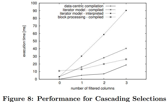
微基准测试
这里实现了四种不同的场景,都是基于HyPer的,包含以数据为中心的编译、以及迭代风格(编译、解释),以及块风格的
数据布局和大小都是完全一样
1
2
3
|
select count(*)
from orderline
where ol_o_id>0 and ol_d_id>0 and ol_w_id>0
|
总体来看,迭代的解释非常慢,改成编译方式就快很多了
块风格的更快,最快的是code-gen
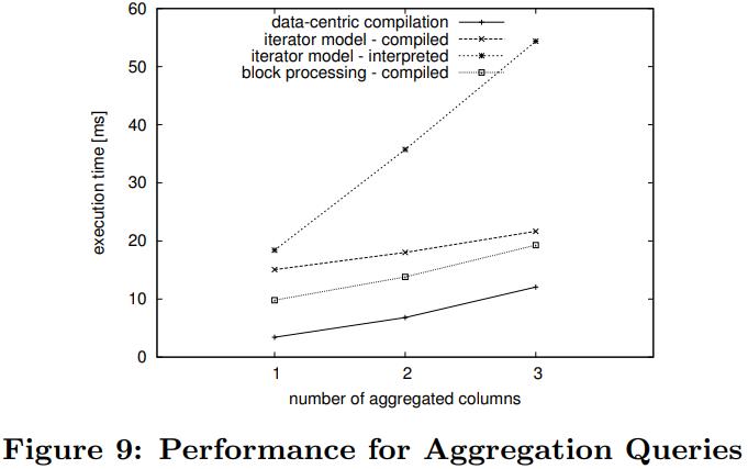
另一个SQL
1
2
|
select sum(ol_o_id*ol_d_id*ol_w_id)
from orderline
|
结果如下,code-gen以数据为中心基本达到了内存带宽上限,在不提升硬件的情况下,性能几乎不可能再提升了
优化设置
使用 g++编译
1
|
-O3 -fgcse-las -funsafe-loop-optimizations.
|
MonetDB会加上:
如果开启了 -funroll-loops,之后又开启了 -fweb 则会影响寄存器分配
对于LLVM编译器,我们通过手动调度优化通道来使用自定义优化级别。精确的级联是
1
2
3
4
5
6
|
llvm::createInstructionCombiningPass()
llvm::createReassociatePass()
llvm::createGVNPass()
llvm::createCFGSimplificationPass()
llvm::createAggressiveDCEPass()
llvm::createCFGSimplificationPass()
|
参考